Multi_R_Designer Tutorial

---

This option is helpful to estimate one or several properties available in the Multi_R_Designer simulator with a complete knowledge of the selected models. Moreover, the simulation results can be saved in a .csv file which can be used with other data processing softwares. If you have already created the frame of user's file, go to the STEP 3.

STEP 1:

• Select Reactor/Trickle bed from the main menu if this option was not chosen before.
• Select Simulation/Start new simulation from the main menu or press .
• A Simulator: Trickle bed dialog window is opened. Go to Frictional pressure drop, choose the desired unit in the Unit field.
• In the Model field, click on the pencil .  Select models available to predict  in the Frictional pressure drop window. All models can be selected by activating the Use heading, or the user can select only some models with the check boxes (see STEP 1 and STEP 2 in section: Frame of user's file).

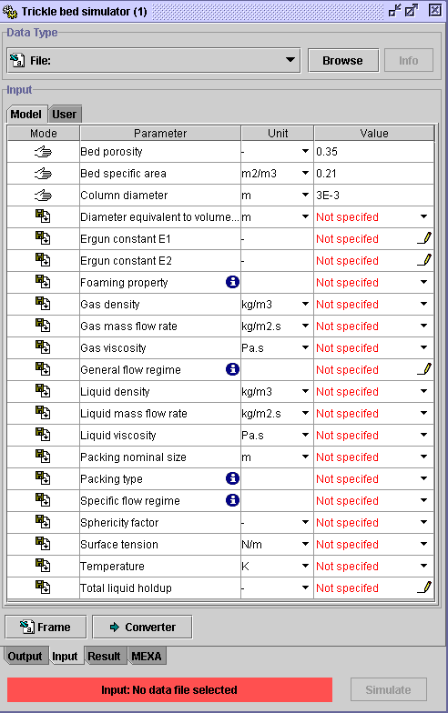
• Select the Input tab at the bottom of the Simulator:Trickle bed dialog window in order to establish what are the required inputs for the application of the models selected in STEP 1.

• Three options are offered to the user relatively to the way of introducing data or inputs in the simulator: Manual, File and User Database.

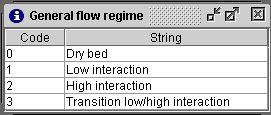
• Some inputs necessitate codes (  ). Consequently, the user must enter the code in the corresponding entry. To know the codes, press(  )

STEP 4:

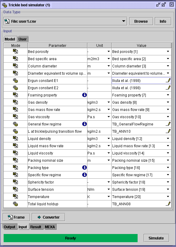
• In this example, user1.csv file contains the inputs on which the simulations will be performed. If a User database has already been prepared, the third option may be chosen (see STEP 6). For the two latter cases, find the desired file using Browse.

• Individual columns in user1.csv are automatically assigned to the correct inputs.
• Inputs not available in sample.csv can be estimated if the symbol  (see STEP 3 and STEP 4 in section: Frame of user's file)
• Click on Simulate to run the simulation.

STEP 6:

• If User database is chosen, find the user database using Browse.
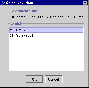
• The user can perform simulations for the whole user database or for one set as shown in the figure below (user1 or user2, see section User database, STEP 5). To select both sets, press the Shift button on the keyboard.

STEP 7:

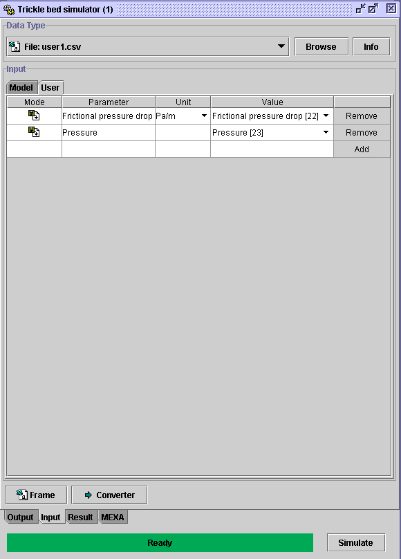
• In this case also, required inputs for the selected models are automatically assigned except those which are not found. Models are available to estimate those inputs when the symbol  is indicated.
• The user can add additional variables in the result's file by selecting the User tab.
• Click on Simulate to run the simulation.

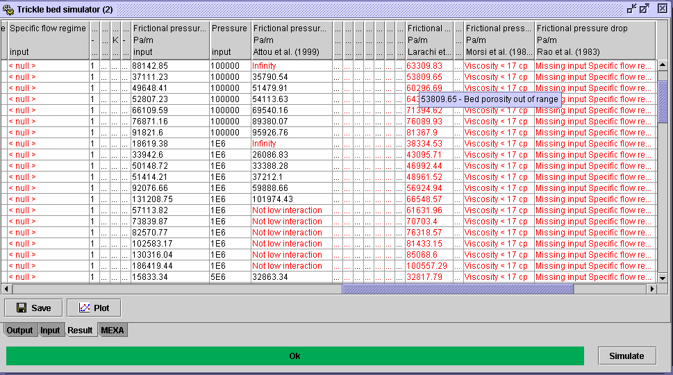
• Once the simulations are finished, click on Result. The results tabulation is revealed.
• The columns are identified with the variables input or the model's name for the simulated outputs.
• Variables (inputs or outputs) estimated by a model are identified. By clicking on these column headings, an information panel about this model is displayed.
• If the inputs are not available in any way, < null > is written in the appropriate cell (in this example: Specific flow regime). If the missing input is essential for the application of a model, a Missing input ... is written in the corresponding model's output cell (Rao et al. (1983) for example).
• Output values displayed in red means that at least one input is out of the validity range. Focusing the red values gives the reason why it is considered invalid. For example, in the figure below, the data 53809.65 predicted by the Larachi et al. model is out of range for bed porosity. These invalid data are symbolized by open dots when plotted.
• If the model is not applicable (Attou et al. model for low interaction flow regime), an appropriate comment is given (Not low interaction).

STEP 9:

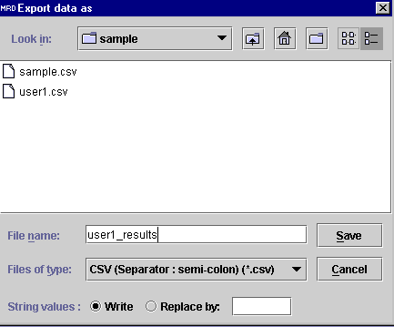
• The result's file can be saved using the Save option. Two formats are available: semi-colon separator ( .csv) and tabulation separator (.txt).
• These format allow the manipulation of the file in other data processing softwares (Windows editor, Microsoft Excel, ....).

• For graphical representation of the simulation results, click on Plot.
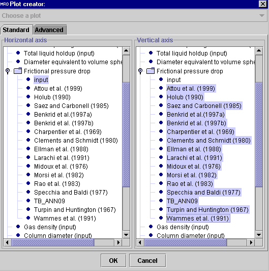
• In the Plot Creator dialog window, the user must choose a variable for the Horizontal Axis (left panel) and another for the Vertical Axis (right panel).
• The symbol  offers the possibility to choose several items. Click on the knob to see what they are.
• As shown in the figure below, a parity plot of one or several models' predictions is obtained when Experimental in the Frictional pressure drop folder is selected as the Horizontal axis (left panel) while the models' predictions are set in the Vertical axis (right panel).

STEP 11:

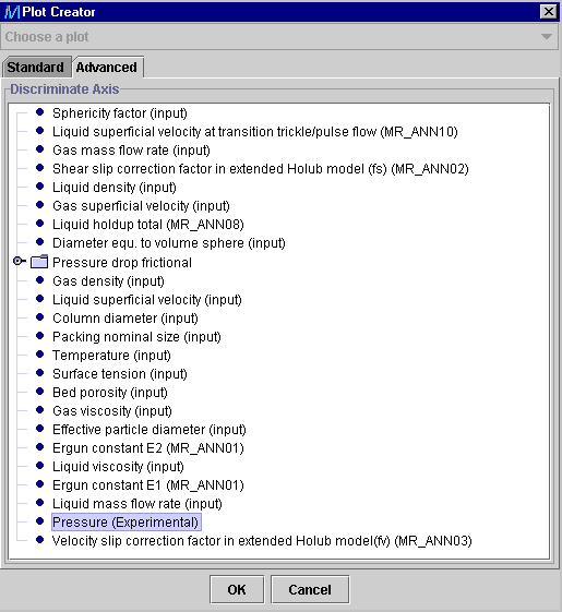
• In the Advanced tab, an additional variable can be selected for subsequent quantitative discrimination. In this example, the Experimental operating Pressure from the Frictional pressure drop folder is chosen.

STEP 12:

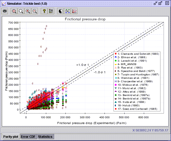
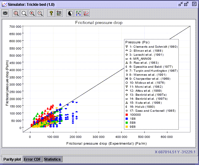
• Press OK to display the parity plot. Each colored set is associated to a model in the Legend panel. Graph properties, such as the axis scaling, tittle, legend, color and symbols shape ..., can be changed in the Edit chart properties dialog window .
• Press  and select the desired points on the graph in order to obtain the corresponding XY coordinates.

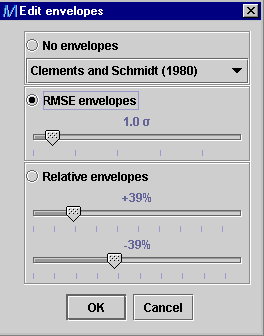
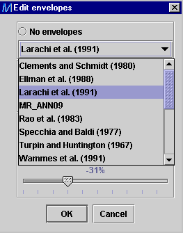
• As default, the RMSE envelopes based on the first correlation/model predictions presented in the legend are drawn on the parity plot. The user can modify the envelopes by choosing in the Edit envelopes dialog window  between No envelopes, RMSE envelopes or Relative envelopes (AARE). The RMSE envelopes and Relative envelopes are based on the correlations/model chosen from the list below the No envelopes option.

• Hollow symbols indicate that at least one model input to calculate the predicted frictional pressure drop is out of range of validity. To remove the invalid data from the diagram, press on Show only valid points .
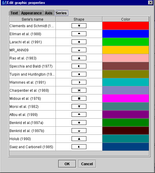
• The color and shape of the series associated to a model may also be changed (see figure below). Press  and select Series tab.

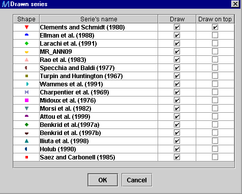
• The user can remove one or several series from the graph (right click on the legend). Deselect the undesired models in the Drawn series dialog window shown below.

STEP 13:

• Two discrimination methods can be achieved on graphs, based on:
• qualitative variable such as the flow regime, packing, fluid nature and any coded variables
• quantitative variable such as the operating pressure selected in STEP 11.
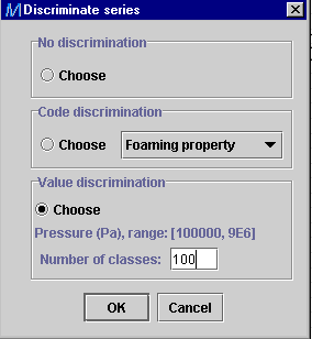
• Click on Discriminate series  and choose the desired option. For the quantitative discrimination, the min-max value range for pressure is given (min: 100000 and 9E6). The user can write in the box the number of equally-divided classes for discrimination (i.e. 100).

STEP 14:

• Once the discrimination on valid points is done, one can see the prediction efficiency of models represented by a symbol shape for each pressure range represented by a color.

STEP 15a:

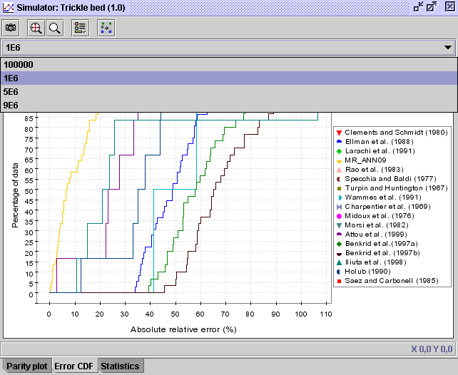
• The performance of the models represented in the Parity plot can be depicted in cumulative distribution function diagrams (click on Error CDF tab) for each model (identified by a color) and each discriminated parameter. Curves can be represented for all data or valid points only .

STEP 15b:

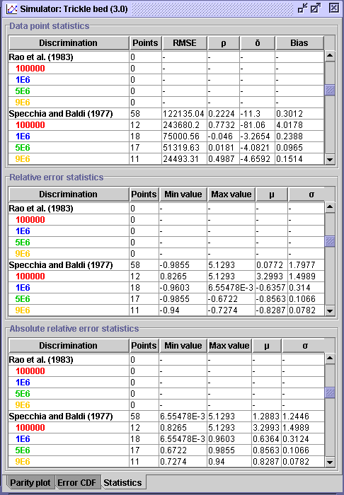
• Statistical evaluation is summarized in a table divided in three sections: Data point statistics, Relative error statistics and Absolute relative error statistics. The user may complete his study based on the statistical information that suit him the best.

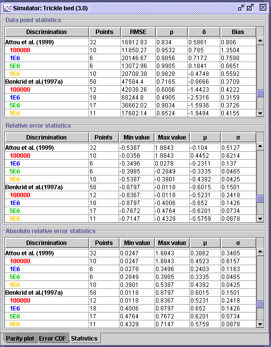In the Discrimination field, the model name and discriminated parameter are listed for the three sections. The definitions of the statistical parameters are given in the graphical representation section in the quick guide manual. The number of points predicted by the model and the number of points associated to the discriminated parameter are given in the second column. From this table, many observations can be drawn. As indicated in the Results' table (STEP 8), the Rao et al (1983) model was not simulated. Consequently, 0 is written in the Points field. When the model is only valid for a specific conditions such as the Specchia and Baldi (1977) model (applicable for high interaction flow regime), statistical parameters were obtained based on 58 data sets only (left figure above). In the right figure above, one can see that the Attou et al. (1999) model is applicable on 38 data sets (low interaction flow regime) and it is mostly effective for cases operated at 1 MPa in terms of average absolute error ((AARE) = 24%,  = 11.6% and  = 98.5%). The Benkrid et al. (1997a) model applicable on 58 points (high interaction flow regime) has a good correlation coefficient for 5 and 9 MPa operation whereas the AARE is the lowest for 0.1 MPa operation. Nevertheless, its performance is better than Specchia and Baldi' s model.

Other conclusions can be drawn from the statistical tabulation. Comparing other models and other discriminated parameters would finally enable the user to select the best model matching the studied experimental conditions. An other tool presented below: MEXA, can be also used in the same perspective.

STEP 16:

• At any time during the study, the user can save and print the project.

Multi_R_Designer Tutorial