Multi_R_Designer Tutorial

---

1) Start a new query .

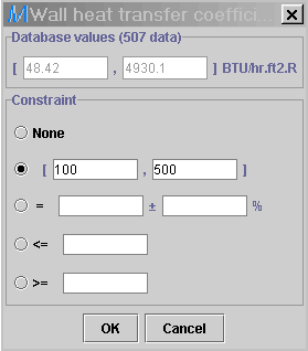
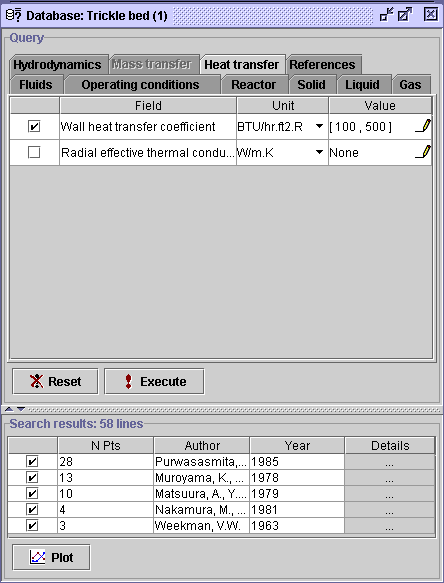
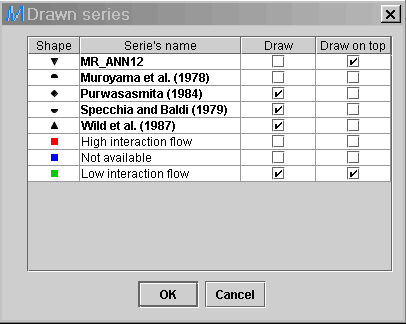
2) In the Heat transfer tab, check the Wall heat transfer coefficient and change the units from the default W/m2.K to BTU/hr.ft2.R. In the Value field dialog window, enter 100 and 500 in the range [,] option. Press OK, then Execute.
 

3) In the Reactor tab, select Beads from the Packing type field, then Execute (41 data sets remain).

4) In the Packing material field, select Glass, then Execute. It leaves the actual Search results list with 40 data sets fulfilling the entered specifications.

5) Select the Plot button  to open the plot creator.

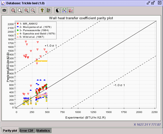
6) In the Horizontal axis panel (Standard tab), click on the knob corresponding to Heat transfer, then on the knob corresponding to Wall heat transfer coefficient.  Highlight Experimental.

7) In the Vertical axis panel, click on Heat transfer, then on Wall heat transfer coefficient. Select all available correlations on this aspect, namely the MR_ANN12, Muroyama et al. (1978), Purwasasmita (1984), Specchia and Baldi (1979) and Wild et al. (1987) correlations. Press OK. The following diagram is created.
 

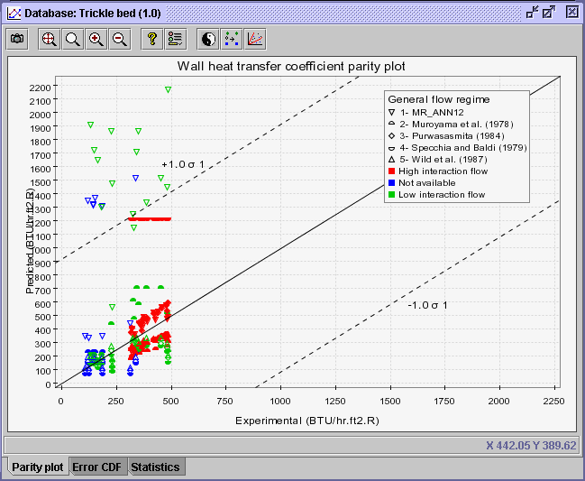
8) Select the Discriminate series  button and choose General flow regime from the Code discrimination combo box . PressOK. Three discriminated series appear (High interaction flow, Not available, Low interaction flow). Not available means that the general flow regime is unknown for the specified data sets.
 

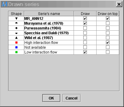
9) Now unselect the discriminated series (High interaction & Not available) to study the performance of correlations for low interaction flow operation only. Right click on the legend and uncheck the corresponding boxes in the Draw field. Then, unselect the last 3 correlations (Purwasasmita (1984), Specchia and Baldi (1979) and Wild et al. (1987)) to alleviate the diagram. Press OK.
 

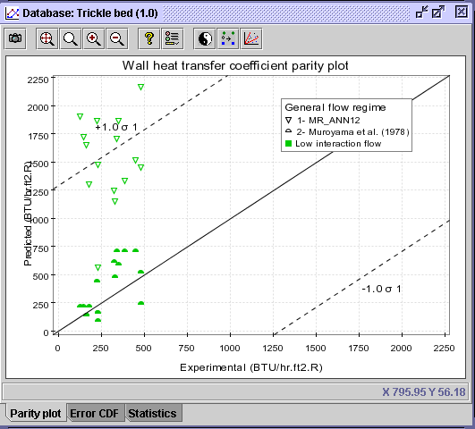CONCLUSION #1: At first glance, the Muroyama et al. (1978) correlation presents better prediction accuracy for low interaction flow operation. On the other hand, the MR_ANN12 correlation, being mostly invalid for these data sets presents out of range predictions.

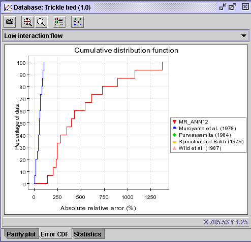
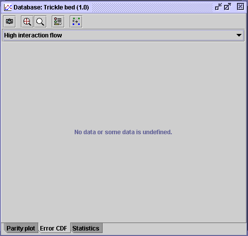
10) The CDF curve corroborates the fact that Muroyama et al. (1978) is much superior. In the Error CDF panel, change the Low interaction flow option for High interaction flow in the combo box. Since this series was deactivated in the legend, no CDF diagram could be created.
 

11) Return to the Parity plot panel, and click on the legend. Inverse the correlations selection in the Draw field. Press OK.
 

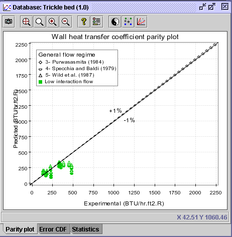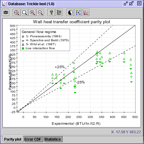
12) This diagram is inconclusive from the actual point of view. First, in the Edit envelopes  dialog window, select Purwasasmita (1984) in the combo box . Press OK. Then, in the Edit graphic properties  dialog window (Axis tab), unselect the Scale automatically option and change the Maximum range value for 500 in both the Horizontal axis and Vertical axis tabs.

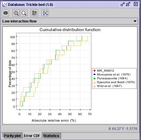
13) The resulting diagram does not produce much better conclusions. However, in the Error CDF panel, the Wild et al. (1987) seems to have a slight advantage over the others.
 

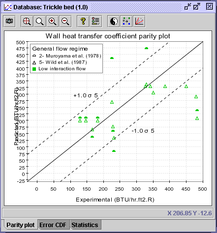
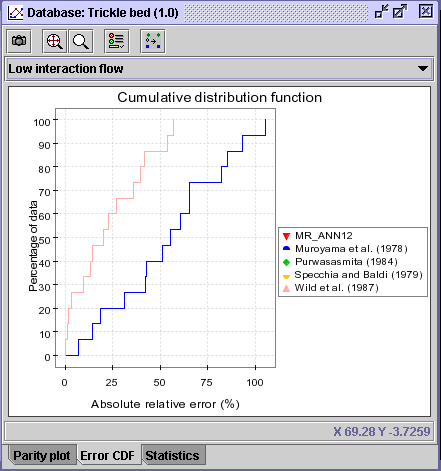
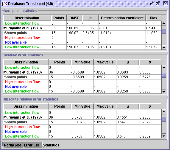
14) Return to the legend in the Parity plot, and select the Muroyama et al. (1978) and Wild et al. (1987) correlations for the final analysis. Press OK. Then, change the envelopes for the RMSE envelopes based on Wild et al. (1987) results. Press OK.
 
 

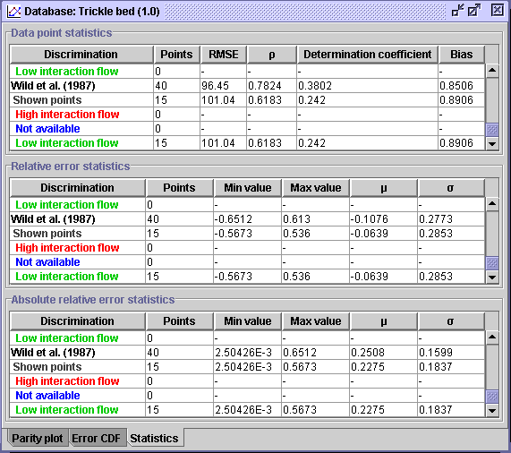CONCLUSION #2: The figures shown above (CDF and Statistics) exhibit without a doubt that the Wild et al. (1987) correlation (AARE = 22.75 %) predicting wall heat transfer coefficients is more potent than Muroyama et al. (1978) correlation (AARE = 54.7%) for low interaction flow regime operation.

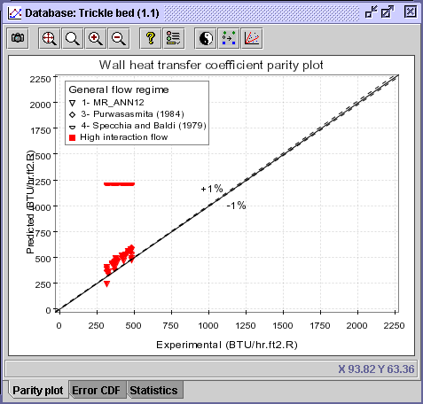
15) For the h_w analysis (high interaction flow experiments), return to the legend (right click) in the Parity plot, unselect Low interaction flow and re-select High interaction flow. Press OK.
 

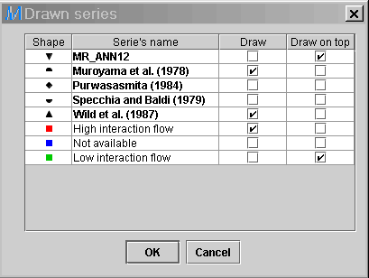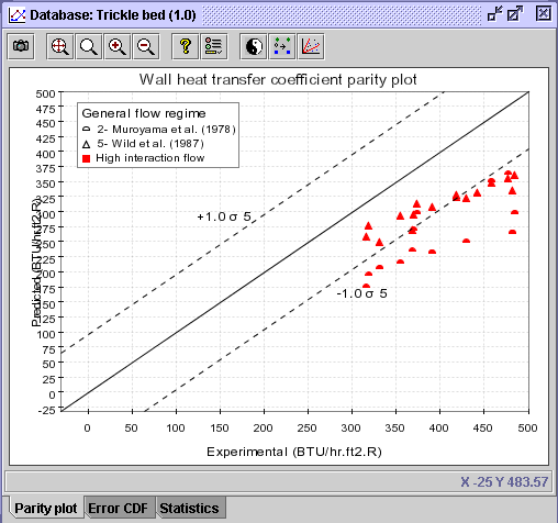CONCLUSION #3: It appears that both correlations, which are predicting fairly well h_w for low interaction flow experiments, simply under-predict h_w for high interaction flow operation. Consequently, the other 3 correlations should be further analysed with the same data points.

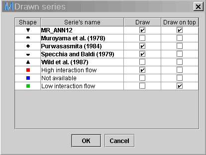
16) Right click on the legend in the parity plot and inverse the selections in the Draw field for the correlations only. Press OK.
 

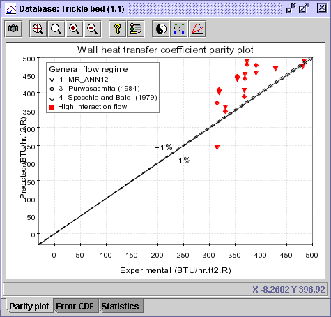17) Press the Zoom To Fit  button to reset the axes scale.

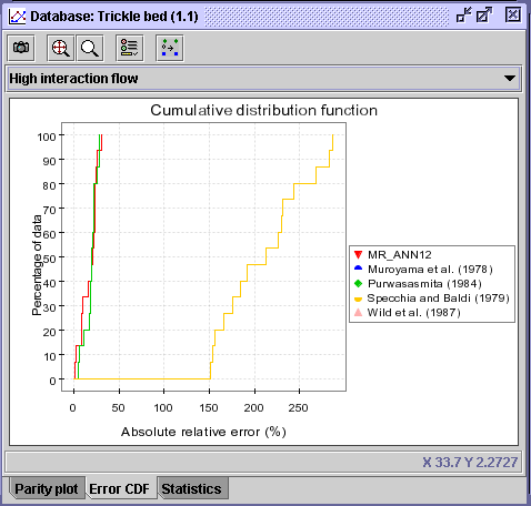
18) The Error CDF panel shows that the Specchia and Baldi (1979) is inappropriate for the prediction of h_w at high interaction flow operation. As for the other 2 correlations, they seem fairly comparable.
 
 

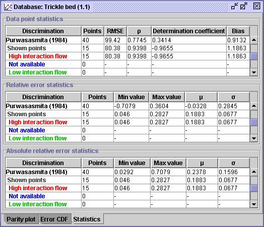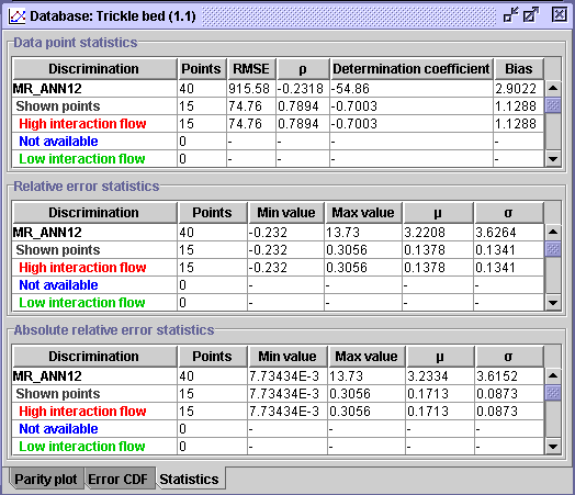
CONCLUSION #4: From a statistical point of view, the MR_ANN12 correlation (AARE = 17.13%) seems slightly more efficient if not equivalent to the Purwasasmita (1984) correlation (AARE = 18.83%) for predicting wall heat transfer coefficients associated with high interaction flow operation.

Multi_R_Designer Tutorial