| Multi_R_Designer Tutorial |
1) Using the diagram from
the Conclusion in Sub-problem
5.2, an interpolation between the series (Red dot: 13272 &
Blue dot: 26544) at G = 1000 lb/ft2/hr is necessary.
Using the zooming option ![]() ,
reduce the X and Y axes scale by selecting a square ranging between 500<X<1500
and 350<Y<700. A new zoomed diagram will be created.
,
reduce the X and Y axes scale by selecting a square ranging between 500<X<1500
and 350<Y<700. A new zoomed diagram will be created.
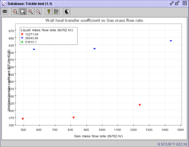 |
CONCLUSION #1: At X = 1000 for a gasoil mass flow rate of 15000 lb/ft2/hr, the Y value or hw can be approximated between 425-475 BTU/hr/ft2/R. Purwasasmita also worked in similar conditions with kerosene. For comparison, hw will be approximated with the same conditions for kerosene flow.
2) Beforehand, reduce the actual diagram window (now you got 2 diagrams waiting to be printed) and return to the Query index.
3) In the Liquid tab, unselect the box corresponding to Liquid viscosity, then Execute.
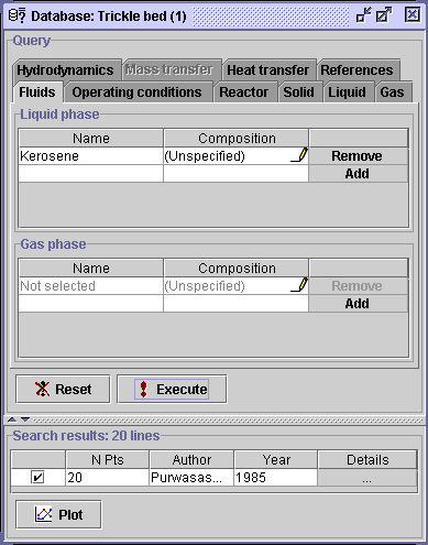
4) In the Fluids tab, click on the Add button in the Liquid phase panel.
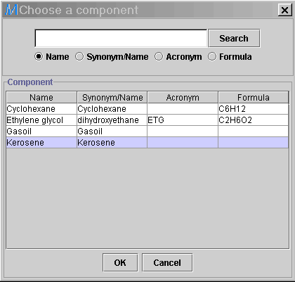
5) In the Choose a component
dialog window, highlight Kerosene and press OK, then Execute.
A
total of 20 data sets which deals with kerosene in the liquid phase
are extracted.
 |
 |
6) Select the Plot
button ![]() .
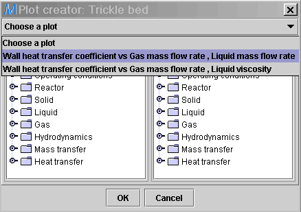
In the Choose a plot combo box, choose Wall heat transfer coefficient
(Vertical
axis) vs Gas mass flow rate (Horizontal axis), Liquid mass flow
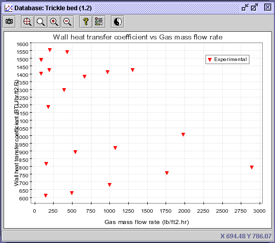
rate (Discriminate). The following diagram will be created.
.
In the Choose a plot combo box, choose Wall heat transfer coefficient
(Vertical
axis) vs Gas mass flow rate (Horizontal axis), Liquid mass flow
rate (Discriminate). The following diagram will be created.
 |
 |
7) Select the Discriminate
series button ![]() and check the Value discrimination option. Write 10 in the
Number
of classes entry. Press OK.
and check the Value discrimination option. Write 10 in the
Number
of classes entry. Press OK.
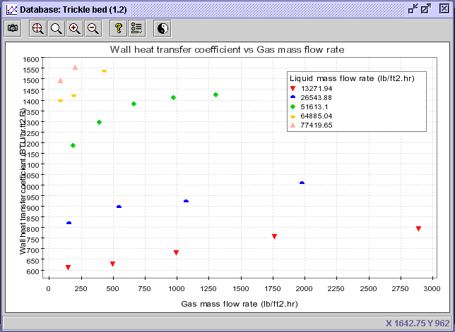 |
CONCLUSION #2: From the latter diagram, at X = 1000 for a kerosene mass flow rate of 15000 lb/ft2/hr, the Y value or h w can be approximated between 700-800 BTU/hr/ft2 /R compared to 425-475 BTU/hr/ft2/R for gasoil flow with the same operating conditions.
| Multi_R_Designer Tutorial |